Let’s pretend you recently installed R (a software to do statistical computing), you have a text collection you would like to analyze or classify and some time to lose. Here are a few quick commands that could get you a little further. I also write this kind of cheat sheet in order to remember a set of useful tricks and packages I recently gathered and from which I thought they could help others too.
Letter frequencies
In this example I will use a series of characteristics (or features) extracted from a text collection, more precisely the frequency of each letter from a to z (all lowercase). By the way, it goes as simple as that using Perl and regular expressions (provided you have a $text variable):
my @letters = ("a" .. "z");
foreach my $letter (@letters) {
    my $letter_count = () = $text =~ /$letter/gi;
    printf "%.3f", (($letter_count/length($text))*100);
}
First tests in R
After having started R (‘R’ command), one usually wants to import data. In this case, my file type is TSV (Tab-Separated Values) and the first row contains only describers (from ‘a’ to ‘z’), which comes at hand later. This is done using the read.table command.
alpha <- read.table("letters_frequency.tsv", header=TRUE, sep="\t")
Then, after examining a glimpse of the dataset (summary(alpha)), for instance to see if everything looks fine, one may start to calculate and visualize a correlation matrix:
correlation_matrix <- cor(alpha)
install.packages("lattice") # if it is not already there
library(lattice)
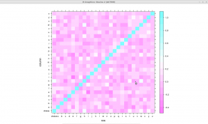
levelplot(correlation_matrix)
Here is the result, it works out of the box even if you did not label your data, I will use the “choice” column later. The colors do not fully match my taste but this is a good starting point.
 Correlation matrix (or ‘heat map’) of letter frequencies in a collection
of texts written in English.
You may click on the image to enlarge it (sorry for the mouse pointer on the map), but as far as I am concerned there are no strong conclusions to draw from this visualization, let alone the fact that the letters frequencies are not distributed randomly. Prettier graphs can be made, see for instance this thread.
Models and validation: a few guidelines
Now, let’s try to build a model that fits the data. To do this you need a reference, in this case the choice column, which is a binary choice: ‘1’ or ‘yes’ and ‘0’ or ‘no’, whether annotated or determined randomly. You may also try to model the frequency of the letter ‘a’ using the rest of the alphabet.
You could start from a hypothesis regarding the letter frequency, like “the frequency of the letter ‘e’ is of paramount importance to predict the frequency of the letter ‘a’”. You may also play around with the functions in R, come up with something interesting and call it ‘data-driven analysis’.
One way or another, what you have to do seems simple: find a baseline to compare your results to, find a model and optimize it, compare and evaluate the results. R is highly optimized to perform these tasks and the computation time should not be the issue here. Nevertheless, there are a lot of different methods available in R, and to choose one that suits your needs might require a considerable amount of time.
Example 1: Regression Analysis
Going a step further, I will start with regression analysis, more precisely with linear regression, i.e. lm(), since it may be easier to understand what the software does.
Other models of this family include the generalized linear model, glm(), and the generalized additive
model, gam() with the mgcv package. Their operation is similar.
The following commands define a baseline, select all the features, print a summary and show a few plots:
alpha.lm.baseline <- lm(choice ~ 1 , data = alpha)
alpha.lm <- lm(choice ~ . , data = alpha)
summary(alpha.lm)
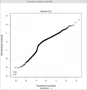
plot(alpha.lm)`
‘.’ means ‘every other column’, another possibility is ‘column_a + column_b + column_d’ etc.
 A plot of model coverage (or ‘fit’) and so-called residuals
In order to determine if the components (features) of the models are relevant (concerning regression analysis), the commands exp(), coef() and coefint() may be interesting, as they give hints whether a given model is supposed to generalize well or not.
Selecting features
You may also be able to do more (or at least as much as you already do) with less, by deleting features that bear no statistical relevance. There are a lot of ways to select features, all the more since this issue links to a field named dimensionality reduction.
Fortunately, R has a step() function which reduces gradually the number of features and stops if no statistically predictable improvement has been reached. However, fully automatic processing is not the best way to find a core of interesting features, one usually has to assess which framework to work with depending on the situation.
Frequently mentioned techniques include lasso sequences, ridge regression, leaps and bounds, or selection using the caret package. Please note that this list is not exhaustive at all…
To get a glimpse of another framework (same principles but another scientific tradition), I think principal components analysis (using princomp()) is worth a look.
This accessible paper presents different issues related to this topic and summarizes several techniques addressing it:
- An Introduction to Variable and Feature Selection, Isabelle Guyon and André Elisseeff, Journal of Machine Learning Research 3 (2003), pp. 1157-1182.
Evaluating the results
In many scientific fields, cross-validation is an acknowledged evaluation method. There are a lot of slightly different ways to perform such a validation, see for instance this compendium.
I will just describe two easy steps suiting the case of a binary choice. Firstly, drawing a prediction table usually works, even if it is not the shortest way, and enables to see what evaluating means. Please note that this example is bad, as on one hand the model is only evaluated once and the other hand the evaluation is performed on its own training data:
alpha.pred <- predict.lm(alpha.glm)
alpha.pred <- ifelse(alpha.pred <= 0, 0, 1)
table(alpha.pred, alpha$choice, dnn=c("predicted","observed"))
sum(diag(alpha.tab))/sum(logdata.tab)
The DAAG package (Data Analysis And Graphics) allows for quicker ways to estimate results AND perform a cross-validation on a few kinds of linear models using binary choices, for example with this command:
cv.binary(alpha.lm)
Example 2: Decision Trees
Decision trees are another way to discover more about data. By the way, the package used in this example, rpart (recursive partitioning and regression trees) also supports regression algorithms.
library(rpart)
alpha.tree <- rpart(choice ~ . , data = alpha, method="anova")
plotcp(alpha.tree)`
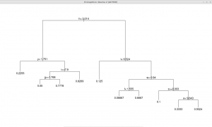
Because the anova method was applied, this is actually a regression tree. The “control” option should be used to prevent the tree to grow unnecessarily deep or broad.
The printcp() command enables to see the variables actually used in tree construction, which may be interesting. Making a summary() can output lots of text, as all the tree is detailed node by node. This is easy to understand, since the algorithm takes decisions based on statistical regularities, in that case letter frequencies are used to split the input into many scenarios (the terminal nodes of a tree), such as “if ‘u’ is under a certain limit and ‘d’ above another, than we look at the frequency of ‘f’ and ‘j’ and take another decision”, etc.

plot(alpha.tree)
text(alpha.tree)`
All the decisions are accessible, this is called a ‘white box’ model. Nonetheless, if decision tree learning has advantages, it also bears limitations.
A few links to go further
- CRAN Task View: Machine Learning & Statistical Learning
- Resources to help you learn and use R
- An introduction to R
- Data Mining Algorithms In R (Wikibook, sometimes incomplete or a bit old)